Logistic Regression

Regression for a qualitative binary response variable $(Y_i = 0$ or $1)$. The explanatory variables can be either quantitative or qualitative.

Use Logistic Regression to predict true - false with numeric values

Simple Logistic Regression Model

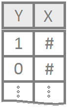
Regression for a qualitative binary response variable $(Y_i = 0$ or $1)$ using a single (typically quantitative) explanatory variable.

Overview

The probability that $Y_i = 1$ given the observed value of $x_i$ is called $\pi_i$ and is modeled by the equation

Math Code

$$
  P(Y_i = 1|\, x_i) = \frac{e^{\beta_0 + \beta_1 x_i}}{1+e^{\beta_0 + \beta_1 x_i}} = \pi_i
$$

$P($ The “P” stands for “Probability that…” $Y_i$ The response variable. The “i” denotes that this is the y-value for individual “i”, where “i” is 1, 2, 3,… and so on up to $n$, the sample size. $= 1$ Equals 1… This states that we are assuming that the probability that the response variable $Y_i$ is a 1 for the current individual. $| x_i)$ Given $x_i$… in other words, the “|” says “given” and $x_i$ means the x-value of the current individual. $=$ Equals sign. $\displaystyle\frac{e^{\beta_0 + \beta_1 x_i}}{1 + e^{\beta_0 + \beta_1 x_i}}$ The logistic regression equation where $e=2.71828...$ is the “natural constant” number and $\beta_0$ is the y-intercept and $\beta_1$ is teh slope. $= \pi_i$ The $\pi_i$ stands for the probability of individual $i$ having a y-value equal to 1 given their $x_i$ value. It is the short hand notation for $P(Y_i = 1 |x_i)$. (It is NOT the number 3.14…)

The coefficents $\beta_0$ and $\beta_1$ are difficult to interpret directly. Typicall $e^{\beta_0}$ and $e^{\beta_1}$ are interpreted instead. The value of $e^{\beta_0}$ or $e^{\beta_1}$ denotes the relative change in the odds that $Y_i=1$. The odds that $Y_i=1$ are $\frac{\pi_i}{1-\pi_i}$.

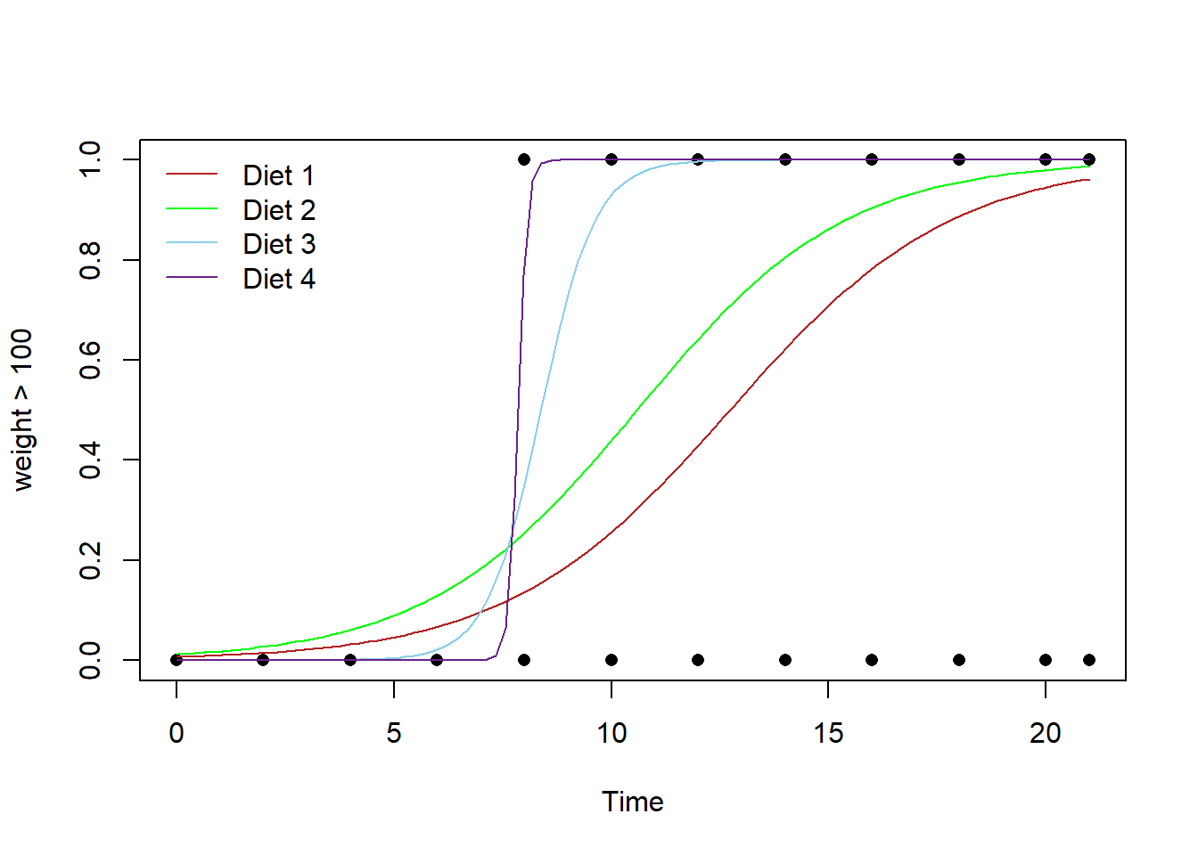
Examples: challenger mouse

R Instructions

Console Help Command: ?glm()

To perform a logistic regression in R use the commands

YourGlmName This is some name you come up with that will become the R object that stores the results of your logistic regression glm() command. <- This is the “left arrow” assignment operator that stores the results of your glm() code into YourGlmName. glm( glm( is an R function that stands for “General Linear Model”. It works in a similar way that the lm( function works except that it requires a family= option to be specified at the end of the command. Y Y is your binary response variable. It must consist of only 0’s and 1’s. Since TRUE’s = 1’s and FALSE’s = 0’s in R, Y could be a logical statement like (Price > 100) or (Animal == “Cat”) if your Y-variable wasn’t currently coded as 0’s and 1’s. ~ The tilde symbol ~ is used to tell R that Y should be treated as a function of the explanatory variable X. X, X is the explanatory variable (typically quantitative) that will be used to explain the probability that the response variable Y is a 1. data = NameOfYourDataset,
NameOfYourDataset is the name of the dataset that contains Y and X. In other words, one column of your dataset would be called Y and another column would be called X. family=binomial) The family=binomial command tells the glm( function to perform a logistic regression. It turns out that glm can perform many different types of regressions, but we only study it as a tool to perform a logistic regression in this course.
summary(YourGlmName) The summary command allows you to print the results of your logistic regression that were previously saved in YourGlmName.

Example output from a regression. Hover each piece to learn more.

Call:
glm(formula = am ~ disp, family = binomial, data = mtcars) This is simply a statement of your original glm(…) “call” that you made when performing your regression. It allows you to verify that you ran what you thought you ran in the glm(…).

Deviance Residuals: EXPLANATION.
Min -1.5651 “min” gives the value of the residual that is furthest below the regression line. Ideally, the magnitude of this value would be about equal to the magnitude of the largest positive residual (the max) because the hope is that the residuals are normally distributed around the line.	1Q -0.6648 “1Q” gives the first quartile of the residuals, which will always be negative, and ideally would be about equal in magnitude to the third quartile.	Median -0.2460 “Median” gives the median of the residuals, which would ideally would be about equal to zero. Note that because the regression line is the least squares line, the mean of the residuals will ALWAYS be zero, so it is never included in the output summary. This particular median value of -0.2460 is a little smaller than zero than we would hope for and suggests a right skew in the data because the mean (0) is greater than the median (-0.2460) witnessing the residuals are right skewed. This can also be seen in the maximum being much larger in magnitude than the minimum.	3Q 0.7276 “3Q” gives the third quartile of the residuals, which would ideally would be about equal in magnitude to the first quartile. In this case, it is pretty close, which helps us see that the first quartile of residuals on either side of the line is behaving fairly normally.	Max 2.2691 “Max” gives the maximum positive residuals, which would ideally would be about equal in magnitude to the minimum residual. In this case, it is much larger than the minimum, which helps us see that the residuals are likely right skewed.

Coefficients: Notice that in your glm(…) you used only $Y$ and $X$. You did type out any coefficients, i.e., the $\beta_0$ or $\beta_1$ of the regression model. These coefficients are estimated by the glm(…) function and displayed in this part of the output along with standard errors, t-values, and p-values.
	Estimate To learn more about the “Estimates” of the “Coefficients” see the “Explanation” tab, “Estimating the Model Parameters” section for details.	Std. Error To learn more about the “Standard Errors” of the “Coefficients” see the “Explanation” tab, “Inference for the Model Parameters” section.	z value EXPLANATION	Pr(>\|z\|) EXPLANATION
(Intercept) This always says “Intercept” for any glm(…) you run in R. That is because R always assumes there is a y-intercept for your regression function.	2.630849 This is the estimate of the y-intercept, $\beta_0$. It is called $b_0$. It is the value of the log of the odds that $Y_i=1$ when $x_i$ is zero. Remember to use $e^{b_0}$ to interpret this values actual effect on the odds.	1.050170 This is the standard error of $b_0$. It tells you how much $b_0$ varies from sample to sample. The closer to zero, the better.	2.505 EXPLANATION	0.01224 This is the p-value of the test of the hypothesis that $\beta_0 = 0$. It measures the probability of observing a t-value as extreme as the one observed. To compute it yourself in R, use `pt(-abs(your t-value), df of your regression)*2`.	* This is called a “star”. One star means significant at the 0.1 level of $\alpha$.
disp This is always the name of your X-variable in your glm(Y ~ X, …).	-0.014604 This is the estimate of the slope, $\beta_1$. It is called $b_1$. It is the change in the log of the odds that $Y_i = 1$ as X is increased by 1 unit. Remember to use $e^{b_1}$ to compute the actual effect on the odds.	0.005168 This is the standard error of $b_1$. It tells you how much $b_1$ varies from sample to sample. The closer to zero, the better.	-2.826 EXPLANATION	0.00471 This is the p-value of the test of the hypothesis that $\beta_1 = 0$. To compute it yourself in R, use `pt(-abs(your t-value), df of your regression)*2`	** This is called a “star”. Three stars means significant at the 0.001 level of $\alpha$.

---

Signif. codes: 0 ‘***’ 0.001 ‘**’ 0.01 ‘*’ 0.05 ‘.’ 0.1 ‘ ’ 1 These “codes” explain what significance level the p-value is smaller than based on how many “stars” * the p-value is labeled with in the Coefficients table above.

(Dispersion parameter for binomial family taken to be 1) EXPLANATION

Null Deviance: EXPLANATION

43.230 EXPLANATION

on 31 degrees of freedom EXPLANATION

Residual deviance: EXPLANATION

29.732 EXPLANATION

on 30 degrees of freedom This is $n-p$ where $n$ is the sample size and $p$ is the number of parameters in the regression model. In this case, there is a sample size of 32 and two parameters, $\beta_0$ and $\beta_1$, so 32-2 = 30.

AIC: EXPLANATION

33.732 EXPLANATION

Number of Fisher Scoring iterations: EXPLANATION

5 EXPLANATION

To check the goodness of fit of a logistic regression model when there are many replicated $x$-values use the command

pchisq( The pchisq command allows you to compute p-values from the chi-squared distribution. residual deviance, The residual deviance is shown at the bottom of the output of your summary(YourGlmName) and should be typed in here as a number like 25.3. df for residual deviance, The df for the residual deviance is also shown at the bottom of the output of your summary(YourGlmName). lower.tail=FALSE) This command ensures you find the probability of the chi-squared distribution being as extreme or more extreme than the observed value of residual deviance.

## [1] 0.479439

To check the goodness of fit of a logistic regression model where there are few or no any replicated $x$-values

library(ResourceSelection) This loads the ResourceSelection R package so that you can access the hoslem.test() function. You may need to run the code: install.packages(“ResourceSelection”) first.
hoslem.test( This R function performs the Hosmer-Lemeshow Goodness of Fit Test. See the “Explanation” file to learn about this test. YourGlmName YourGlmName is the name of your glm(…) code that you created previously. $y, ALWAYS type a “y” here. This gives you the actual binary (0,1) y-values of your logistic regression. The goodness of fit test will compare these actual values to your predicted probabilities for each value in order to see if the model is a “good fit.” YourGlmName YourGlmName is the name you used to save the results of your glm(…) code. $fitted, ALWAYS type “fitted” here. This gives you the fitted probabilities $\pi_i$ of your logistic regression. g=10) The “g=10” is the default option for the value of g. The g is the number of groups to run the goodness of fit test on. Just leave it at 10 unless you are told to do otherwise. Ask your teacher for more information if you are interested.

## 
##  Hosmer and Lemeshow goodness of fit (GOF) test
## 
## data:  myglm$y, myglm$fitted
## X-squared = 5.7327, df = 8, p-value = 0.6771

Plot the Regression

plot( The plot function allows us to draw a scatterplot where the y-axis is only 0’s or 1’s and the x-axis is quantitative. Y Y should be some logical statement like Fail > 0 or sex == “B” or height < 68. In other words, Y needs to be a collection of 0’s and 1’s. ~ The tilde is read “Y on X.” X, X is some quantitative variable. data= Tell the plot which data set to use. X and Y are columns of that data set. YourDataSet The name of your data set. ) Closing parenthesis for plot(…) function.
curve( A function in R that draws a “curve” on a plot. Using add=TRUE puts the curve onto the current plot. exp( This allows you to compute e to the power of something. So exp(1) = e, exp(2) = e^2 and so on. $b_0$ + This is the “Intercept” estimate from your logistic regression summary output. $b_1$ This is the slope estimate from your logistic regression summary output. *x The curve function demands you ALWAYS use a lower-case “x” in this function. ) Closing parenthesis. / The division symbol. (1 + Required for the formula. exp($b_0$ + $b_1$*x) This needs to match exactly the first version of this statement. ), Closing parenthesis for the denominator. add = TRUE) This makes the curve be added to the current plot. If it is left out, the curve will be drawn in a new plot.

ggplot( EXPLANATION. data, EXPLANATION. aes( EXPLANATION. X, EXPLANATION. Y EXPLANATION. ) Closing parenthesis for aes(…) function. ) Closing parenthesis for ggplot(…) function. + EXPLANATION.
geom_point( EXPLANATION. ) EXPLANATION. + EXPLANATION.
geom_smooth( EXPLANATION. method= EXPLANATION. “glm”, EXPLANATION. method.args = EXPLANATION. list( EXPLANATION. family = EXPLANATION. “binomial”), EXPLANATION. se = EXPLANATION. FALSE EXPLANATION. ) EXPLANATION. + EXPLANATION.
theme_bw() EXPLANATION.

## `geom_smooth()` using formula 'y ~ x'

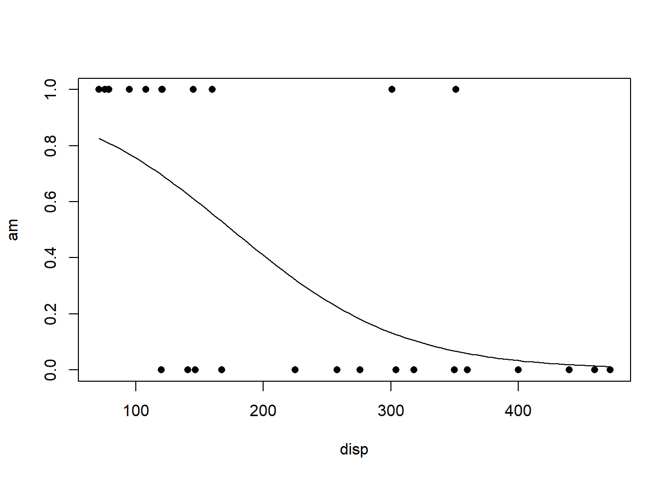
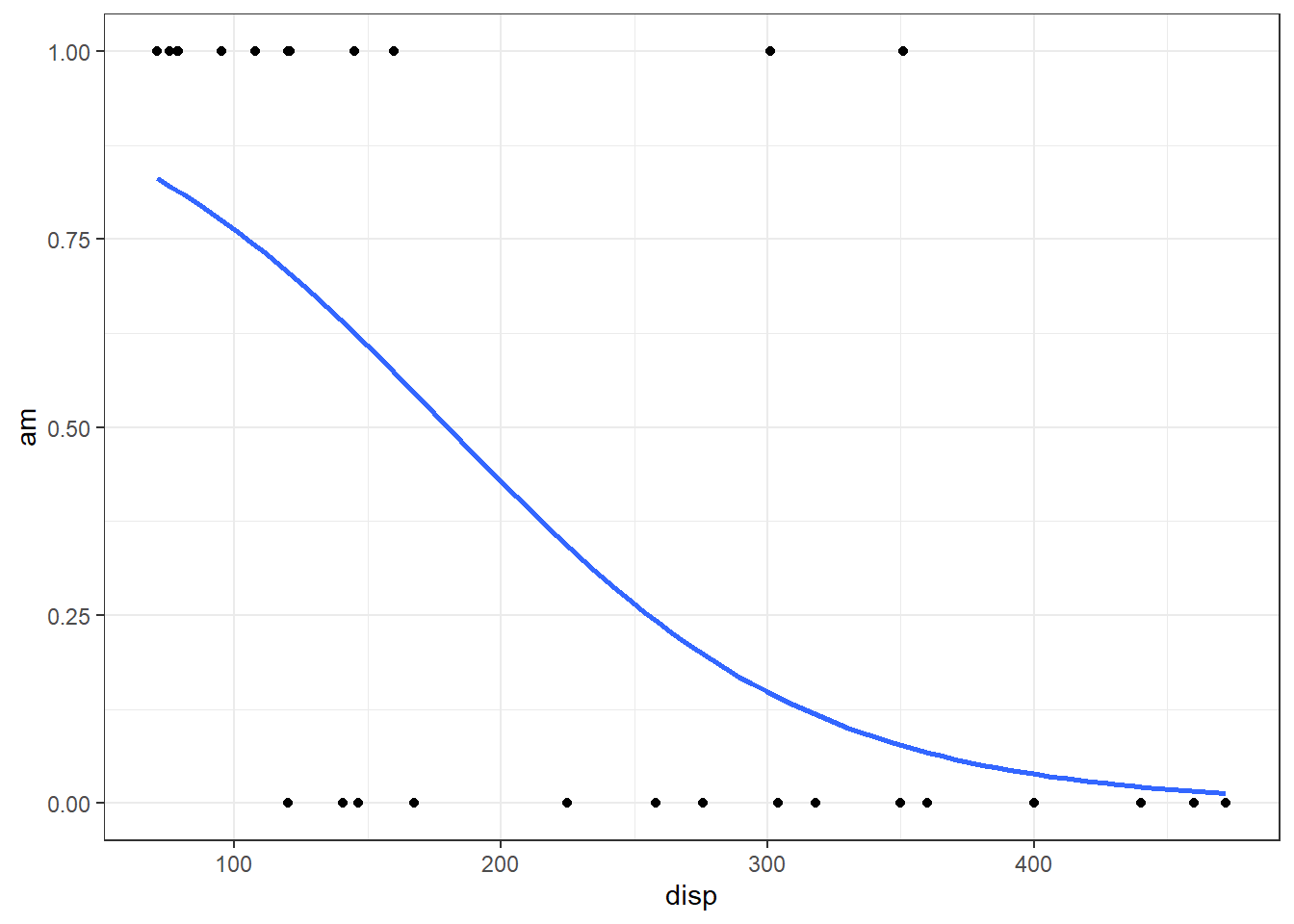
To predict the probability that $Y_i=1$ for a given $x$-value, use the code

predict( The predict() function allows us to use the regression model that was obtained from glm() to predict the probability that $Y_i = 1$ for a given $X_i$. YourGlmName, YourGlmName is the name of the object you created when you performed your logistic regression using glm(). newdata = The newdata = command allows you to specify the x-values for which you want to obtain predicted probabilities that $Y_i=1$. data.frame(xVariableName = someNumericValue), The xVariableName is the same one you used in your glm(y ~ x, …) statement for “x”. Input any desired value for the “someNumericValue” spot. Then, the predict code uses the logistic regression model equation to calculate a predicted probability that $Y_i = 1$ for the given $x_i$ value that you specify. type = “response”) The type = “response” options specifies that you want predicted probabilities. There are other options available. See ?predict.glm for details.

myglm <- glm(am ~ disp, data = mtcars, family = binomial)
predict(myglm, newdata = data.frame(disp = 200), type = "response")

##         1 
## 0.4280016

Explanation

Simple Logistic Regression is used when

the response variable is binary $(Y_i=0$ or $1)$, and
there is a single explanatory variable $X$ that is typically quantitative but could be qualitative (if $X$ is binary or ordinal).

The Model

Since $Y_i$ is binary (can only be 0 or 1) the model focuses on describing the probability that $Y_i=1$ for a given scenario. The probability that $Y_i = 1$ given the observed value of $x_i$ is called $\pi_i$ and is modeled by the equation

\[ P(Y_i = 1|\, x_i) = \frac{e^{\beta_0 + \beta_1 x_i}}{1+e^{\beta_0 + \beta_1 x_i}} = \pi_i \]

The assumption is that for certain values of $X$ the probability that $Y_i=1$ is higher than for other values of $X$.

Interpretation

This model for $\pi_i$ comes from modeling the log of the odds that $Y_i=1$ using a linear regression, i.e., \[ \log\underbrace{\left(\frac{\pi_i}{1-\pi_i}\right)}_{\text{Odds for}\ Y_i=1} = \underbrace{\beta_0 + \beta_1 x_i}_{\text{linear regression}} \] Beginning to solve this equation for $\pi_i$ leads to the intermediate, but important result that \[ \underbrace{\frac{\pi_i}{1-\pi_i}}_{\text{Odds for}\ Y_i=1} = e^{\overbrace{\beta_0 + \beta_1 x_i}^{\text{linear regression}}} = e^{\beta_0}e^{\beta_1 x_i} \] Thus, while the coefficients $\beta_0$ and $\beta_1$ are difficult to interpret directly, $e^{\beta_0}$ and $e^{\beta_1}$ have a valuable interpretation. The value of $e^{\beta_0}$ is interpreted as the odds for $Y_i=1$ when $x_i = 0$. It may not be possible for a given model to have $x_i=0$, in which case $e^{\beta_0}$ has no interpretation. The value of $e^{\beta_1}$ denotes the proportional change in the odds that $Y_i=1$ for every one unit increase in $x_i$.

Notice that solving the last equation for $\pi_i$ results in the logistic regression model presented at the beginning of this page.

Hypothesis Testing

Similar to linear regression, the hypothesis that \[ H_0: \beta_1 = 0 \\ H_a: \beta_1 \neq 0 \] can be tested with a logistic regression. If $\beta_1 = 0$, then there is no relationship between $x_i$ and the log of the odds that $Y_i = 1$. In other words, $x_i$ is not useful in predicting the probability that $Y_i = 1$. If $\beta_1 \neq 0$, then there is information in $x_i$ that can be utilized to predict the probability that $Y_i = 1$, i.e., the logistic regression is meaningful.

Checking Model Assumptions

The model assumptions are not as clear in logistic regression as they are in linear regression. For our purposes we will focus only on considering the goodness of fit of the logistic regression model. If the model appears to fit the data well, then it will be assumed to be appropriate.

Deviance Goodness of Fit Test

If there are replicated values of each $x_i$, then the deviance goodness of fit test tests the hypotheses \[ H_0: \pi_i = \frac{e^{\beta_0 + \beta_1 x_i}}{1+e^{\beta_0 + \beta_1 x_i}} \] \[ H_a: \pi_i \neq \frac{e^{\beta_0 + \beta_1 x_i}}{1+e^{\beta_0 + \beta_1 x_i}} \]

Hosmer-Lemeshow Goodness of Fit Test

If there are very few or no replicated values of each $x_i$, then the Hosmer-Lemeshow goodness of fit test can be used to test these same hypotheses. In each case, the null assumes that logistic regression is a good fit for the data while the alternative is that logistic regression is not a good fit.

Prediction

One of the great uses of Logistic Regression is that it provides an estimate of the probability that $Y_i=1$ for a given value of $x_i$. This probability is often referred to as the risk that $Y_i=1$ for a certain individual. For example, if $Y_i=1$ implies a person has a disease, then $\pi_i=P(Y_i=1)$ represents the risk of individual $i$ having the disease based on their value of $x_i$, perhaps a measure of their cholesterol or some other predictor of the disease.

Multiple Logistic Regression Model

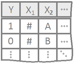
Logistic regression for multiple explanatory variables that can either be quantitative or qualitative or a mixture of the two.

Overview

The probability that $Y_i = 1$ given the observed data $(x_{i1},\ldots,x_{ip})$ is called $\pi_i$ and is modeled by the equation

\[ P(Y_i = 1|\, x_{i1},\ldots,x_{ip}) = \frac{e^{\beta_0 + \beta_1 x_{i1} + \ldots + \beta_p x_{ip}}}{1+e^{\beta_0 + \beta_1 x_{i1} + \ldots + \beta_p x_{ip} }} = \pi_i \]

The coefficents $\beta_0,\beta_1,\ldots,\beta_p$ are difficult to interpret directly. Typically $e^{\beta_k}$ for $k=0,1,\ldots,p$ is interpreted instead. The value of $e^{\beta_k}$ denotes the relative change in the odds that $Y_i=1$. The odds that $Y_i=1$ are $\frac{\pi_i}{1-\pi_i}$.

Examples: GSS

R Instructions

Console Help Command: ?glm()

To perform a logistic regression in R use the commands

YourGlmName This is some name you come up with that will become the R object that stores the results of your logistic regression glm() command. <- This is the “left arrow” assignment operator that stores the results of your glm() code into YourGlmName. glm( glm( is an R function that stands for “General Linear Model”. It works in a similar way that the lm( function works except that it requires a family= option to be specified at the end of the command. Y Y is your binary response variable. It must consist of only 0’s and 1’s. Since TRUE’s = 1’s and FALSE’s = 0’s in R, Y could be a logical statement like (Price > 100) or (Animal == “Cat”) if your Y-variable wasn’t currently coded as 0’s and 1’s. ~ The tilde symbol ~ is used to tell R that Y should be treated as a function of the explanatory variable X. X1 X1 is the first explanatory variable (typically quantitative) that will be used to explain the probability that the response variable Y is a 1. * EXPLANATION X2 X2 is second the explanatory variable either quantitative or qualitative that will be used to explain the probability that the response variable Y is a 1. …, In theory, you could have many other explanatory variables, interaction terms, or even squared, cubed, or other transformations of terms added to this model. data = NameOfYourDataset,
NameOfYourDataset is the name of the dataset that contains Y and X. In other words, one column of your dataset would be called Y and another column would be called X. family=binomial) The family=binomial command tells the glm( function to perform a logistic regression. It turns out that glm can perform many different types of regressions, but we only study it as a tool to perform a logistic regression in this course.
summary(YourGlmName) The summary command allows you to print the results of your logistic regression that were previously saved in YourGlmName.

Example output from a regression. Hover each piece to learn more.

Call:
glm(formula = weight > 100 ~ Time*Diet, family = binomial, data = ChickWeight) This is simply a statement of your original glm(…) “call” that you made when performing your regression. It allows you to verify that you ran what you thought you ran in the glm(…).

Deviance Residuals: EXPLANATION.
Min -2.9446 “min” gives the value of the residual that is furthest below the regression line. Ideally, the magnitude of this value would be about equal to the magnitude of the largest positive residual (the max) because the hope is that the residuals are normally distributed around the line.	1Q -0.2364 “1Q” gives the first quartile of the residuals, which will always be negative, and ideally would be about equal in magnitude to the third quartile.	Median 0.0000 “Median” gives the median of the residuals, which would ideally would be about equal to zero. Note that because the regression line is the least squares line, the mean of the residuals will ALWAYS be zero, so it is never included in the output summary.	3Q 0.2776 “3Q” gives the third quartile of the residuals, which would ideally would be about equal in magnitude to the first quartile. In this case, it is pretty close, which helps us see that the first quartile of residuals on either side of the line is behaving fairly normally.	Max 1.9968 “Max” gives the maximum positive residuals, which would ideally would be about equal in magnitude to the minimum residual. In this case, it is much larger than the minimum, which helps us see that the residuals are likely right skewed.

Coefficients: Notice that in your glm(…) you used only $Y$ and $X$. You did type out any coefficients, i.e., the $\beta_0$ or $\beta_1$ of the regression model. These coefficients are estimated by the glm(…) function and displayed in this part of the output along with standard errors, t-values, and p-values.
	Estimate To learn more about the “Estimates” of the “Coefficients” see the “Explanation” tab, “Estimating the Model Parameters” section for details.	Std. Error To learn more about the “Standard Errors” of the “Coefficients” see the “Explanation” tab, “Inference for the Model Parameters” section.	z value EXPLANATION	Pr(>\|z\|) EXPLANATION
(Intercept) This always says “Intercept” for any glm(…) you run in R. That is because R always assumes there is a y-intercept for your regression function.	-4.97603 This is the estimate of the y-intercept, $\beta_0$. It is called $b_0$. It is the average y-value when X is zero.	0.65316 This is the standard error of $b_0$. It tells you how much $b_0$ varies from sample to sample. The closer to zero, the better.	-7.618 EXPLANATION	2.57e-14 This is the p-value of the test of the hypothesis that $\beta_0 = 0$. It measures the probability of observing a t-value as extreme as the one observed. To compute it yourself in R, use `pt(-abs(your t-value), df of your regression)*2`.	*** This is called a “star”. Three stars means significant at the 0.01 level of $\alpha$.
Time This is always the name of your X-variable in your glm(Y ~ X, …).	0.39111 This is the estimate of the slope, $\beta_1$. It is called $b_1$. It is the change in the average y-value as X is increased by 1 unit.	0.04979 This is the standard error of $b_1$. It tells you how much $b_1$ varies from sample to sample. The closer to zero, the better.	7.854 EXPLANATION	4.02e-15 This is the p-value of the test of the hypothesis that $\beta_1 = 0$. To compute it yourself in R, use `pt(-abs(your t-value), df of your regression)*2`	*** This is called a “star”. Three stars means significant at the 0.01 level of $\alpha$.
Diet2 This is always the name of your X-variable in your glm(Y ~ X, …).	0.58283 This is the estimate of the change in the intercept, $\beta_2$. It is called $b_2$.	1.04061 This is the standard error of $b_2$. It tells you how much $b_2$ varies from sample to sample. The closer to zero, the better.	0.560 EXPLANATION	0.5754 This is the p-value of the test of the hypothesis that $\beta_2 = 0$. To compute it yourself in R, use `pt(-abs(your t-value), df of your regression)*2`
Diet3 This is always the name of your X-variable in your glm(Y ~ X, …).	-8.44476 This is the estimate of the change in the intercept, $\beta_3$. It is called $b_3$.	4.32324 This is the standard error of $b_3$. It tells you how much $b_3$ varies from sample to sample. The closer to zero, the better.	-1.953 EXPLANATION	0.0508 This is the p-value of the test of the hypothesis that $\beta_3 = 0$. To compute it yourself in R, use `pt(-abs(your t-value), df of your regression)*2`	. This is called a period. It means significant at the 0.1 level of $\alpha$.
Diet4 This is always the name of your X-variable in your glm(Y ~ X, …).	-67.41995 This is the estimate of the change in the intercept, $\beta_4$. It is called $b_4$.	3768.10023 This is the standard error of $b_4$. It tells you how much $b_4$ varies from sample to sample. The closer to zero, the better.	-0.018 EXPLANATION	0.9857 This is the p-value of the test of the hypothesis that $\beta_2 = 0$. To compute it yourself in R, use `pt(-abs(your t-value), df of your regression)*2`
Time:Diet2 This is always the name of your X-variable in your glm(Y ~ X, …).	0.02391 This is the estimate of the change in the slope, $\beta_5$. It is called $b_5$.	0.08679 This is the standard error of $b_5$. It tells you how much $b_5$ varies from sample to sample. The closer to zero, the better.	0.275 EXPLANATION	0.7830 This is the p-value of the test of the hypothesis that $\beta_2 = 0$. To compute it yourself in R, use `pt(-abs(your t-value), df of your regression)*2`
Time:Diet3 This is always the name of your X-variable in your glm(Y ~ X, …).	1.20955 This is the estimate of the change in the slope, $\beta_6$. It is called $b_6$.	0.51249 This is the standard error of $b_6$. It tells you how much $b_6$ varies from sample to sample. The closer to zero, the better.	2.360 EXPLANATION	0.0183 This is the p-value of the test of the hypothesis that $\beta_2 = 0$. To compute it yourself in R, use `pt(-abs(your t-value), df of your regression)*2`	* This is called a “star”. One star means significant at the 0.05 level of $\alpha$.
Time:Diet4 This is always the name of your X-variable in your glm(Y ~ X, …).	8.83168 This is the estimate of the change in the slope, $\beta_7$. It is called $b_7$.	471.01259 This is the standard error of $b_7$. It tells you how much $b_7$ varies from sample to sample. The closer to zero, the better.	0.019 EXPLANATION	0.9850 This is the p-value of the test of the hypothesis that $\beta_2 = 0$. To compute it yourself in R, use `pt(-abs(your t-value), df of your regression)*2`

---

(Dispersion parameter for binomial family taken to be 1) EXPLANATION

Null Deviance: EXPLANATION

800.44 EXPLANATION

on 577 degrees of freedom EXPLANATION

Residual deviance: EXPLANATION

256.30 EXPLANATION

on 570 degrees of freedom This is $n-p$ where $n$ is the sample size and $p$ is the number of parameters in the regression model. In this case, there is a sample size of 578 and five parameters, $\beta_0$, $\beta_1$, $\beta_2$, $\beta_3$, $\beta_4$, $\beta_5$,$\beta_6$, and $\beta_7$ so 578-8 = 570.

AIC: EXPLANATION

272.3 EXPLANATION

Number of Fisher Scoring iterations: EXPLANATION

20 EXPLANATION

To check the goodness of fit of a logistic regression model when there are many replicated $x$-values use the command

## [1] 1

To check the goodness of fit of a logistic regression model where there are few or no any replicated $x$-values

## 
##  Hosmer and Lemeshow goodness of fit (GOF) test
## 
## data:  myglm$y, myglm$fitted
## X-squared = 18.212, df = 8, p-value = 0.0197

To predict the probability that $Y_i=1$ for a given $x$-value, use the code

predict( The predict() function allows us to use the regression model that was obtained from glm() to predict the probability that $Y_i = 1$ for a given $X_i$. YourGlmName, YourGlmName is the name of the object you created when you performed your logistic regression using glm(). newdata = The newdata = command allows you to specify the x-values for which you want to obtain predicted probabilities that $Y_i=1$. NewDataFrame, Typically, NewDataFrame is created in real time using the data.frame( X1 = c(Value 1, Value 2, …), X2 = c(Value 1, Value 2, …), …) command. You should see the GSS example file for an example of how to use this function. type = “response”) The type = “response” options specifies that you want predicted probabilities. There are other options available. See ?predict.glm for details.

##         1 
## 0.7314498

Plot the Regression

b EXPLANATION. <- EXPLANATION. mylm EXPLANATION. $ EXPLANATION. coefficients EXPLANATION.
palette( EXPLANATION. c( EXPLANATION. “SomeColor”, EXPLANATION. “DifferentColor”)) EXPLANATION.
plot( EXPLANATION. Y EXPLANATION. ~ EXPLANATION. $X_1$, EXPLANATION. data = YourDataSet, EXPLANATION. pch = 16) EXPLANATION.
curve( EXPLANATION. exp( EXPLANATION. (b[1]+ EXPLANATION. b[2]) EXPLANATION. *x) EXPLANATION. / EXPLANATION. (1+ EXPLANATION. exp( EXPLANATION. b[1]+ EXPLANATION. b[2] EXPLANATION. *x)), EXPLANATION. col = palette()[1], EXPLANATION. add = TRUE) EXPLANATION.
curve( EXPLANATION. exp( EXPLANATION. (b[1]+ EXPLANATION. b[3]) EXPLANATION. +(b[2]+ EXPLANATION. b[4]) EXPLANATION. *x) EXPLANATION. / EXPLANATION. (1+ EXPLANATION. exp( EXPLANATION. (b[1]+ EXPLANATION. b[3]) EXPLANATION. +(b[2]+ EXPLANATION. b[4]) EXPLANATION. *x)), EXPLANATION. col = palette()[2], EXPLANATION. add = TRUE) EXPLANATION.
legend( EXPLANATION. “position”, EXPLANATION. legend = EXPLANATION. c(“Level 1”, “Level 2”), EXPLANATION. col = palette(), EXPLANATION. lty = 1, EXPLANATION. bty = EXPLANATION. ‘n’) EXPLANATION.

ggplot( EXPLANATION. data, EXPLANATION. aes( EXPLANATION. $X_1$, EXPLANATION. Y EXPLANATION. ) Closing parenthesis for aes(…) function. ) Closing parenthesis for ggplot(…) function. + EXPLANATION.
geom_point( EXPLANATION. ) EXPLANATION. + EXPLANATION.
geom_smooth( EXPLANATION. method= EXPLANATION. “glm”, EXPLANATION. method.args = EXPLANATION. list( EXPLANATION. family = EXPLANATION. “binomial”), EXPLANATION. aes( EXPLANATION. color = $X_2$) EXPLANATION. se = EXPLANATION. FALSE EXPLANATION. ) EXPLANATION. + EXPLANATION.
theme_bw() EXPLANATION.

## `geom_smooth()` using formula 'y ~ x'

Explanation

Multiple Logistic Regression is used when

the response variable is binary $(Y_i=0$ or $1)$, and
there are multiple explanatory variables $X_1,\ldots,X_p$ that can be either quantitative or qualitative.

The Model

Very little changes in multiple logistic regression from Simple Logistic Regression. The probability that $Y_i = 1$ given the observed data $(x_{i1},\ldots,x_{ip})$ is called $\pi_i$ and is modeled by the expanded equation

\[ P(Y_i = 1|\, x_{i1},\ldots,x_{ip}) = \frac{e^{\beta_0 + \beta_1 x_{i1} + \ldots + \beta_p x_{ip}}}{1+e^{\beta_0 + \beta_1 x_{i1} + \ldots + \beta_p x_{ip} }} = \pi_i \]

The assumption is that for certain combinations of $X_1,\ldots,X_p$ the probability that $Y_i=1$ is higher than for other combinations.

Interpretation

The model for $\pi_i$ comes from modeling the log of the odds that $Y_i=1$ using a linear regression, i.e., \[ \log\underbrace{\left(\frac{\pi_i}{1-\pi_i}\right)}_{\text{Odds for}\ Y_i=1} = \underbrace{\beta_0 + \beta_1 x_{i1} + \ldots + \beta_p x_{ip}}_{\text{linear regression}} \] Beginning to solve this equation for $\pi_i$ leads to the intermediate, but important result that \[ \underbrace{\frac{\pi_i}{1-\pi_i}}_{\text{Odds for}\ Y_i=1} = e^{\overbrace{\beta_0 + \beta_1 x_{i1} + \ldots + \beta_p x_{ip}}^{\text{liear regression}}} = e^{\beta_0}e^{\beta_1 x_{i1}}\cdots e^{\beta_p x_{ip}} \] As in Simple Linear Regression, the values of $e^{\beta_0}$, $e^{\beta_1}$, $\ldots$, $e^{\beta_p}$ are interpreted as the proportional change in odds for $Y_i=1$ when a given $x$-variable experiences a unit change, all other variables being held constant.

Checking the Model Assumptions

Diagnostics are the same in multiple logistic regression as they are in simple logistic regression.

Prediction

The idea behind prediction in multiple logistic regression is the same as in simple logistic regression. The only difference is that more than one explanatory variable is used to make the prediction of the risk that $Y_i=1$.

Coefficients: Notice that in your glm(…) you used only \(Y\) and \(X\). You did type out any coefficients, i.e., the \(\beta_0\) or \(\beta_1\) of the regression model. These coefficients are estimated by the glm(…) function and displayed in this part of the output along with standard errors, t-values, and p-values.
	Estimate To learn more about the “Estimates” of the “Coefficients” see the “Explanation” tab, “Estimating the Model Parameters” section for details.	Std. Error To learn more about the “Standard Errors” of the “Coefficients” see the “Explanation” tab, “Inference for the Model Parameters” section.	z value EXPLANATION	Pr(>\|z\|) EXPLANATION
(Intercept) This always says “Intercept” for any glm(…) you run in R. That is because R always assumes there is a y-intercept for your regression function.	2.630849 This is the estimate of the y-intercept, \(\beta_0\). It is called \(b_0\). It is the value of the log of the odds that \(Y_i=1\) when \(x_i\) is zero. Remember to use \(e^{b_0}\) to interpret this values actual effect on the odds.	1.050170 This is the standard error of \(b_0\). It tells you how much \(b_0\) varies from sample to sample. The closer to zero, the better.	2.505 EXPLANATION	0.01224 This is the p-value of the test of the hypothesis that \(\beta_0 = 0\). It measures the probability of observing a t-value as extreme as the one observed. To compute it yourself in R, use `pt(-abs(your t-value), df of your regression)*2`.	* This is called a “star”. One star means significant at the 0.1 level of \(\alpha\).
disp This is always the name of your X-variable in your glm(Y ~ X, …).	-0.014604 This is the estimate of the slope, \(\beta_1\). It is called \(b_1\). It is the change in the log of the odds that \(Y_i = 1\) as X is increased by 1 unit. Remember to use \(e^{b_1}\) to compute the actual effect on the odds.	0.005168 This is the standard error of \(b_1\). It tells you how much \(b_1\) varies from sample to sample. The closer to zero, the better.	-2.826 EXPLANATION	0.00471 This is the p-value of the test of the hypothesis that \(\beta_1 = 0\). To compute it yourself in R, use `pt(-abs(your t-value), df of your regression)*2`	** This is called a “star”. Three stars means significant at the 0.001 level of \(\alpha\).

Coefficients: Notice that in your glm(…) you used only \(Y\) and \(X\). You did type out any coefficients, i.e., the \(\beta_0\) or \(\beta_1\) of the regression model. These coefficients are estimated by the glm(…) function and displayed in this part of the output along with standard errors, t-values, and p-values.
	Estimate To learn more about the “Estimates” of the “Coefficients” see the “Explanation” tab, “Estimating the Model Parameters” section for details.	Std. Error To learn more about the “Standard Errors” of the “Coefficients” see the “Explanation” tab, “Inference for the Model Parameters” section.	z value EXPLANATION	Pr(>\|z\|) EXPLANATION
(Intercept) This always says “Intercept” for any glm(…) you run in R. That is because R always assumes there is a y-intercept for your regression function.	-4.97603 This is the estimate of the y-intercept, \(\beta_0\). It is called \(b_0\). It is the average y-value when X is zero.	0.65316 This is the standard error of \(b_0\). It tells you how much \(b_0\) varies from sample to sample. The closer to zero, the better.	-7.618 EXPLANATION	2.57e-14 This is the p-value of the test of the hypothesis that \(\beta_0 = 0\). It measures the probability of observing a t-value as extreme as the one observed. To compute it yourself in R, use `pt(-abs(your t-value), df of your regression)*2`.	*** This is called a “star”. Three stars means significant at the 0.01 level of \(\alpha\).
Time This is always the name of your X-variable in your glm(Y ~ X, …).	0.39111 This is the estimate of the slope, \(\beta_1\). It is called \(b_1\). It is the change in the average y-value as X is increased by 1 unit.	0.04979 This is the standard error of \(b_1\). It tells you how much \(b_1\) varies from sample to sample. The closer to zero, the better.	7.854 EXPLANATION	4.02e-15 This is the p-value of the test of the hypothesis that \(\beta_1 = 0\). To compute it yourself in R, use `pt(-abs(your t-value), df of your regression)*2`	*** This is called a “star”. Three stars means significant at the 0.01 level of \(\alpha\).
Diet2 This is always the name of your X-variable in your glm(Y ~ X, …).	0.58283 This is the estimate of the change in the intercept, \(\beta_2\). It is called \(b_2\).	1.04061 This is the standard error of \(b_2\). It tells you how much \(b_2\) varies from sample to sample. The closer to zero, the better.	0.560 EXPLANATION	0.5754 This is the p-value of the test of the hypothesis that \(\beta_2 = 0\). To compute it yourself in R, use `pt(-abs(your t-value), df of your regression)*2`
Diet3 This is always the name of your X-variable in your glm(Y ~ X, …).	-8.44476 This is the estimate of the change in the intercept, \(\beta_3\). It is called \(b_3\).	4.32324 This is the standard error of \(b_3\). It tells you how much \(b_3\) varies from sample to sample. The closer to zero, the better.	-1.953 EXPLANATION	0.0508 This is the p-value of the test of the hypothesis that \(\beta_3 = 0\). To compute it yourself in R, use `pt(-abs(your t-value), df of your regression)*2`	. This is called a period. It means significant at the 0.1 level of \(\alpha\).
Diet4 This is always the name of your X-variable in your glm(Y ~ X, …).	-67.41995 This is the estimate of the change in the intercept, \(\beta_4\). It is called \(b_4\).	3768.10023 This is the standard error of \(b_4\). It tells you how much \(b_4\) varies from sample to sample. The closer to zero, the better.	-0.018 EXPLANATION	0.9857 This is the p-value of the test of the hypothesis that \(\beta_2 = 0\). To compute it yourself in R, use `pt(-abs(your t-value), df of your regression)*2`
Time:Diet2 This is always the name of your X-variable in your glm(Y ~ X, …).	0.02391 This is the estimate of the change in the slope, \(\beta_5\). It is called \(b_5\).	0.08679 This is the standard error of \(b_5\). It tells you how much \(b_5\) varies from sample to sample. The closer to zero, the better.	0.275 EXPLANATION	0.7830 This is the p-value of the test of the hypothesis that \(\beta_2 = 0\). To compute it yourself in R, use `pt(-abs(your t-value), df of your regression)*2`
Time:Diet3 This is always the name of your X-variable in your glm(Y ~ X, …).	1.20955 This is the estimate of the change in the slope, \(\beta_6\). It is called \(b_6\).	0.51249 This is the standard error of \(b_6\). It tells you how much \(b_6\) varies from sample to sample. The closer to zero, the better.	2.360 EXPLANATION	0.0183 This is the p-value of the test of the hypothesis that \(\beta_2 = 0\). To compute it yourself in R, use `pt(-abs(your t-value), df of your regression)*2`	* This is called a “star”. One star means significant at the 0.05 level of \(\alpha\).
Time:Diet4 This is always the name of your X-variable in your glm(Y ~ X, …).	8.83168 This is the estimate of the change in the slope, \(\beta_7\). It is called \(b_7\).	471.01259 This is the standard error of \(b_7\). It tells you how much \(b_7\) varies from sample to sample. The closer to zero, the better.	0.019 EXPLANATION	0.9850 This is the p-value of the test of the hypothesis that \(\beta_2 = 0\). To compute it yourself in R, use `pt(-abs(your t-value), df of your regression)*2`