Numerical Summaries

There are many ways to numerically summarize data. The fundamental idea is to describe the center, or most probable values of the data, as well as the spread, or the possible values of the data.

Mean

\[ \bar{x} = \frac{\sum_{i=1}^n x_i}{n} \]

Measure of Center | 1 Quantitative Variable

Overview

The “balance point” or “center of mass” of quantitative data. It is calculated by taking the numerical sum of the values divided by the number of values. Typically used in tandem with the standard deviation. Most appropriate for describing the most typical values for relatively normally distributed data. Influenced by outliers, so it is not appropriate for describing strongly skewed data.

R Instructions

To calculate a mean in R use the code:

mean(object)

object must be a quantitative variable, what R calls a “numeric vector.” Usually this is a column from a data set.

Example Code

Hover your mouse over the example codes to learn more.

mean “mean” is an R function used to calculate the mean of data. ( Parenthesis to begin the function. Must touch the last letter of the function. airquality “airquality” is a dataset. Type “View(airquality)” in R to see it. $ The $ allows us to access any variable from the airquality dataset. Temp “Temp” is a quantitative variable (numeric vector) from the “airquality” dataset. )
Closing parenthsis for the mean function.
Press Enter to run the code if you have typed it in yourself. You can also click here to view the output. … Click to View Output.

## [1] 77.88235

Note that the single number showing above is the average Temp from the airquality dataset.

library(tidyverse) tidyverse is an R Package that is very useful for working with data.
airquality airquality is a dataset in R. %>% The pipe operator that will send the airquality dataset down inside of the code on the following line.
group_by( “group_by” is a function from library(tidyverse) that allows us to split the airquality dataset into “little” datasets, one dataset for each value in the “Month” column. Month “Month” is a column from the airquality dataset that can be treated as qualitative. ) Functions must always end with a closing parenthesis. %>% The pipe operator that will send the grouped version of the airquality dataset down inside of the code on the following line.
summarise( “summarise” is a function from library(tidyverse) that allows us to compute numerical summaries on data. aveTemp = “AveTemp” is just a name we made up. It will contain the results of the mean(…) function. mean( “mean” is an R function used to calculate the mean. Temp Temp is a quantitative variable (numeric vector) from the airquality dataset. ) Functions must always end with a closing parenthesis. ) Functions must always end with a closing parenthesis.
Press Enter to run the code. … Click to View Output.

## `summarise()` ungrouping output (override with `.groups` argument)

Month	aveTemp
5	65.55
6	79.1
7	83.9
8	83.97
9	76.9

Note that R calculated the mean Temp for each month in Month from the airquality dataset.

May (5), June (6), July (7), August (8), and September (9), respectively.

Further, note that to get the “nicely formatted” table, you would have to use

library(pander)
airquality %>% 
  group_by(Month) %>%
  summarise(aveTemp = mean(Temp)) %>%
  pander()

Explanation

The mathematical formula used to compute the mean of data is given by the formula to the left. Although the formula looks complicated, all it states is “add all the data values up and divide by the total number of values.” Read on to learn what all the symbols in the formula represent.

Symbols in the Formula

$\bar{x}$ is read “x-bar” and is the symbol typically used for the sample mean, the mean computed on a sample of data from a population.
$\Sigma$, the capital Greek letter “sigma,” is the symbol used to imply “add all of the data values up.”
The $x_i$’s are the data values. The $i$ in the $x_i$ is stated to go from $i=1$ all the way up to $n$. In other words, data value 1 is represented by $x_1$, data value 2: $x_2$, $\ldots$, up through the last data value $x_n$. In general, we just write $x_i$.
$n$ represents the sample size, or number of data values.

Population Mean

When all of the data from a population is available, the population mean is calculated instead of the sample mean. The mathematical formula for the population mean is the same as the formula for the sample mean, but is written with slightly different notation. \[ \mu = \frac{\sum_{i=1}^N x_i}{N} \] Notice that the symbol for the population mean is $\mu$, pronounced “mew,” another Greek letter. (Review your Greek alphabet.) The only other difference between the two formulas is that the sample mean uses a sample of data, denoted by $n$, while the population mean uses all the population data, denoted by $N$.

Physical Interpretation

The mean is sometimes described as the “balance point” of the data. The following example will demonstrate.

Say there are $n=5$ data points with the following values.

$x_1 = 2$
$x_2 = 5$
$x_3 = 6$
$x_4 = 7$
$x_5 = 10$

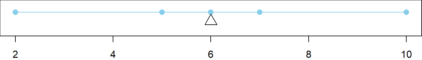
The sample mean is calculated as follows. \[ \bar{x} = \frac{\sum_{i=1}^n x_i}{n} = \frac{2 + 5 + 6 + 7 + 10}{5} = 6 \] If these values were plotted, and an “infinitely thin bar” connected the points, then the bar would “balance” at the mean (the triangle) as shown below.

Middle of the Deviations

The above plot demonstrates that there are equal, but opposite, “sums of deviations” to either side of the mean. Note that a deviation is defined as the distance from the mean to a given point. Thus, $x_1$ has a deviation of -4 from the mean, $x_2$ a deviation of -1, $x_3$ a deviation of 0, $x_4$ a deviation of 1, and $x_5$ a deviation of 4. To the left there is a sum of deviations equal to -5 and on the right, a sum of deviations equal to 5. This can be verified to hold for any scenario.

Effect of Outliers

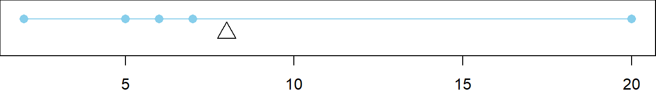
The mean can be strongly influenced by outliers, points that deviate abnormally from the mean. This is shown below by changing $x_5$ to be 20. Note that the deviation of $x_5$ is 12, and the sum of deviations to the left of the mean ($\bar{x}=8$) is $-1 + -2 + -3 + -6 = -12$.

The mean of the altered data

$x_1 = 2$
$x_2 = 5$
$x_3 = 6$
$x_4 = 7$
$x_5 = 20$

is now $\bar{x} = \frac{\sum_{i=1}^n x_i}{n} = \frac{2 + 5 + 6 + 7 + 20}{5} = 8$.

Median

\[ \frac{x_{(n/2)}+x_{(n/2+1)}}{2} \] $\uparrow$ even $n$ odd $\downarrow$

\[ x_{((n+1)/2)} \]

Measure of Center | 1 Quantitative Variable

Overview

The “middle data point,” i.e., the 50$^{th}$ percentile. Half of the data is below the median and half is above the median. Typically used in tandem with the five-number summary to describe skewed data because it is not heavily influenced by outliers, i.e., it is robust. Can also be used with normally distributed data, but the mean and standard deviation are more useful measures in such cases.

R Instructions

To calculate a median in R use the code:

median(object)

object must be a quantitative variable, what R calls a “numeric vector.”

Example Code

median “median” is an R function used to calculate the median of data. ( Parenthesis to begin the function. Must touch the last letter of the function. airquality “airquality” is a dataset. Type “View(airquality)” in R to see it. $ The $ allows us to access any variable from the airquality dataset. Temp “Temp” is a quantitative variable (numeric vector) from the “airquality” dataset. )
Closing parenthsis for the median function.
Press Enter to run the code if you have typed it in yourself. You can also click here to view the output. … Click to View Output.

## [1] 79

Note that the single number showing above is the median Temp from the airquality dataset.

library(tidyverse) tidyverse is an R Package that is very useful for working with data.
airquality airquality is a dataset in R. %>% The pipe operator that will send the airquality dataset down inside of the code on the following line.
group_by( “group_by” is a function from library(tidyverse) that allows us to split the airquality dataset into “little” datasets, one dataset for each value in the “Month” column. Month “Month” is a column from the airquality dataset that can be treated as qualitative. ) Functions must always end with a closing parenthesis. %>% The pipe operator that will send the grouped version of the airquality dataset down inside of the code on the following line.
summarise( “summarise” is a function from library(tidyverse) that allows us to compute numerical summaries on data. medTemp = “medTemp” is just a name we made up. It will contain the results of the median(…) function. median( “median” is an R function used to calculate the median. Temp Temp is a quantitative variable (numeric vector) from the airquality dataset. ) Functions must always end with a closing parenthesis. ) Functions must always end with a closing parenthesis.
Press Enter to run the code. … Click to View Output.

## `summarise()` ungrouping output (override with `.groups` argument)

Month	medTemp
5	66
6	78
7	84
8	82
9	76

Note that R calculated the median Temp for each month in Month from the airquality dataset.

May (5), June (6), July (7), August (8), and September (9), respectively.

Further, to get the nicely formatted table you must use:

library(pander)
airquality %>% 
  group_by(Month) %>%
  summarise(medTemp = median(Temp)) %>%
  pander()

Explanation

The mathematical formula used to compute the median of data depends on whether $n$, the number of data points in the sample, is even or odd.

If $n$ is even, then there is no “middle” data point, so the middle two values are averaged. \[ \text{Median} = \frac{x_{(n/2)}+x_{(n/2+1)}}{2} \]

If $n$ is odd, then the middle data point is the median. \[ \text{Median} = x_{((n+1)/2)} \]

Symbols in the Formula

There is no generally accepted symbol for the median. Sometimes a capital $M$ or even lower-case $m$ is used, but generally the word median is just written out.

$x_{(n/2)}$ represents the data value that is in the $(n/2)^{th}$ position in the ordered list of values. It only exists when $n$ is even.
$x_{(n/2+1)}$ represents the data value that immediately follows the $(n/2)^{th}$ value in the ordered list of values. It only exists when $n$ is even.
$x_{((n+1)/2)}$ represents the data value that is in the $((n+1)/2)^{th}$ position in the ordered list of values. It only exists when $n$ is odd.
$n$ represents the sample size, or number of data values in the sample.

Population Median

When all of the data from a population is available, the population median is calculated by the above formulas with the slight change that $N$, the total number of data values in the population, instead of $n$, the number of values in the sample, is used.

If $N$ is even, then there is no “middle” data point, so the middle two values are averaged. \[ \text{Median} = \frac{x_{(N/2)}+x_{(N/2+1)}}{2} \]

If $N$ is odd, then the middle data point is the median. \[ \text{Median} = x_{((N+1)/2)} \]

Physical Interpretation

The median is the $50^{th}$ percentile of the data.

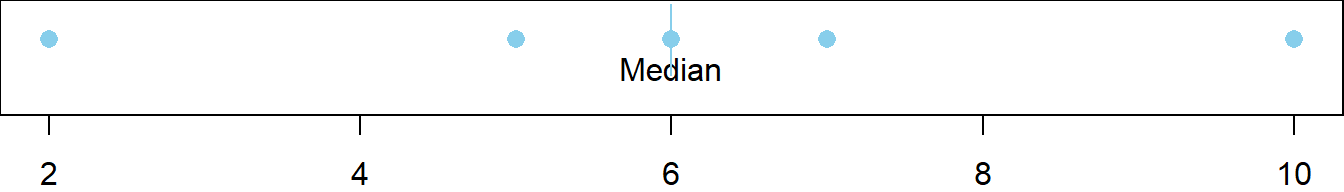
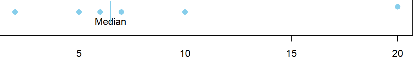
Say there are $n=5$ data points in the sample with the following values.

$x_1 = 2$
$x_2 = 5$
$x_3 = 6$
$x_4 = 7$
$x_5 = 10$

The sample median is calculated as follows. Note that $n=5$ is odd. \[ \text{Median} = x_{((n+1)/2)} = x_{((5+1)/2)} = x_{(3)} = 6 \] When these values are plotted it is clear that exactly 50% of the data (excluding the median) is to either side of the median.

Second Example

Say there was a sixth value in the data set equal to 10, so that $n=6$ is even.

$x_1 = 2$
$x_2 = 5$
$x_3 = 6$
$x_4 = 7$
$x_5 = 10$
$x_6 = 10$

\[ \text{Median} = \frac{x_{(n/2)}+x_{(n/2+1)}}{2} = \frac{x_{(6/2)}+x_{(6/2+1)}}{2} = \frac{x_{(3)}+x_{(4)}}{2} = \frac{6+7}{2} = 6.5 \]

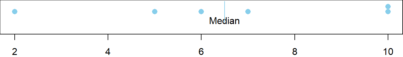
Effect of Outliers

The median is not greatly influenced by outliers. It is said to be robust. This is shown below by changing $x_6$ to be 20, which does not change the value of the median.

Mode

Most

Frequent

Value

Measure of Center | 1 Quantitative or Qualitative Variable

Overview

The most commonly occurring value. There may be more than one mode. Seldom used, but sometimes useful.

R Instructions

R will not calculate a mode directly. However, to tabulate the number of times each value occurs in a dataset, use the code:

table(object)

object can be quantitative or qualitative, but should contain at least one repeated value or table() is not useful.

Example Code

Hover your mouse over the example codes to learn more.

table “table” is an R function used to count how many times each observation occurs in a list of data. ( Parenthesis to begin the function. Must touch the last letter of the function. airquality “airquality” is a dataset. Type “View(airquality)” in R to see it. $ The $ allows us to access any variable from the airquality dataset. Month “Month” is a qualitative variable (technically a numeric vector) from the “airquality” dataset that contains repeated values. )
Closing parenthsis for the function.
Press Enter to run the code if you have typed it in yourself. You can also click here to view the output. … Click to View Output.

## 
##  5  6  7  8  9 
## 31 30 31 31 30

Note that the modes would be 5, 7, and 8 because these months all have the most (31) days in them.

library(tidyverse) tidyverse is an R Package that is very useful for working with data.
airquality airquality is a dataset in R. %>% The pipe operator that will send the airquality dataset down inside of the code on the following line.
group_by( “group_by” is a function from library(tidyverse) that allows us to split the airquality dataset into “little” datasets, one dataset for each value in the “Month” column. Month “Month” is a column from the airquality dataset that can be treated as qualitative. ) Functions must always end with a closing parenthesis. %>% The pipe operator that will send the grouped version of the airquality dataset down inside of the code on the following line.
summarise( “summarise” is a function from library(tidyverse) that allows us to compute numerical summaries on data. aveTemp = mean(Temp), Computes the mean of the Temp column. medTemp = median(Temp), Computes the median of the Temp column. sampleSize = n( ) Counts how many times each Month (the group_by statement) occurs in the dataset. ) Functions must always end with a closing parenthesis.
Press Enter to run the code. … Click to View Output.

## `summarise()` ungrouping output (override with `.groups` argument)

Month	aveTemp	medTemp	sampeSize
5	65.55	66	31
6	79.1	78	30
7	83.9	84	31
8	83.97	82	31
9	76.9	76	30

Note that R calculated the median Temp for each month in Month from the airquality dataset.

May (5), June (6), July (7), August (8), and September (9), respectively.

Further, to get the nicely formatted table you must use:

library(pander)
airquality %>% 
  group_by(Month) %>%
  summarise(aveTemp = mean(Temp), medTemp = median(Temp), sampeSize = n()) %>%
  pander()

Minimum

\[ x_{(1)} \]

Measure of Spread | 1 Quantitative Variable

Overview

The smallest occurring data value. One of the numerical summaries in the five-number summary. Typically not useful on its own. Gives a good feel for the spread in the left tail of the distribution when used with the five-number summary.

R Instructions

To calculate a minimum in R use the code:

min(object)

object must be a quantitative variable, what R calls a “numeric vector.”

Example Code

Hover your mouse over the example codes to learn more.

min “min” is an R function used to calculate the minimum of data. ( Parenthesis to begin the function. Must touch the last letter of the function. airquality “airquality” is a dataset. Type “View(airquality)” in R to see it. $ The $ allows us to access any variable from the airquality dataset. Temp “Temp” is a quantitative variable (numeric vector) from the “airquality” dataset. )
Closing parenthsis for the function.
Press Enter to run the code if you have typed it in yourself. You can also click here to view the output. … Click to View Output.

## [1] 56

Note that the single number showing above is the minimum Temp from the airquality dataset.

library(tidyverse) tidyverse is an R Package that is very useful for working with data.
airquality airquality is a dataset in R. %>% The pipe operator that will send the airquality dataset down inside of the code on the following line.
group_by( “group_by” is a function from library(tidyverse) that allows us to split the airquality dataset into “little” datasets, one dataset for each value in the “Month” column. Month “Month” is a column from the airquality dataset that can be treated as qualitative. ) Functions must always end with a closing parenthesis. %>% The pipe operator that will send the grouped version of the airquality dataset down inside of the code on the following line.
summarise( “summarise” is a function from library(tidyverse) that allows us to compute numerical summaries on data. minTemp = “minTemp” is just a name we made up. It will contain the results of the median(…) function. min( “min” is an R function used to calculate the minimum. Temp Temp is a quantitative variable (numeric vector) from the airquality dataset. ) Functions must always end with a closing parenthesis. ) Functions must always end with a closing parenthesis.
Press Enter to run the code. … Click to View Output.

## `summarise()` ungrouping output (override with `.groups` argument)

Month	minTemp
5	56
6	65
7	73
8	72
9	63

Note that R calculated the minimum Temp for each month in Month from the airquality dataset.

May (5), June (6), July (7), August (8), and September (9), respectively.

Further, to get the nicely formatted table you must use:

library(pander)
airquality %>% 
  group_by(Month) %>%
  summarise(minTemp = min(Temp)) %>%
  pander()

Maximum

\[ x_{(n)} \]

Measure of Spread | 1 Quantitative Variable

Overview

The largest occurring data value. One of the numerical summaries in the five-number summary. Typically not useful on its own. Gives a good feel for the spread in the right tail of the distribution when used in the five-number summary.

R Instructions

To calculate a maximum in R use the code:

max(object)

object must be a quantitative variable, what R calls a “numeric vector.”

Example Code

Hover your mouse over the example codes to learn more.

## [1] 97

Note that the single number showing above is the maximum Temp from the airquality dataset.

library(tidyverse) tidyverse is an R Package that is very useful for working with data.
airquality airquality is a dataset in R. %>% The pipe operator that will send the airquality dataset down inside of the code on the following line.
group_by( “group_by” is a function from library(tidyverse) that allows us to split the airquality dataset into “little” datasets, one dataset for each value in the “Month” column. Month “Month” is a column from the airquality dataset that can be treated as qualitative. ) Functions must always end with a closing parenthesis. %>% The pipe operator that will send the grouped version of the airquality dataset down inside of the code on the following line.
summarise( “summarise” is a function from library(tidyverse) that allows us to compute numerical summaries on data. maxTemp = “maxTemp” is just a name we made up. It will contain the results of the median(…) function. max( “max” is an R function used to calculate the maximum. Temp Temp is a quantitative variable (numeric vector) from the airquality dataset. ) Functions must always end with a closing parenthesis. ) Functions must always end with a closing parenthesis.
Press Enter to run the code. … Click to View Output.

## `summarise()` ungrouping output (override with `.groups` argument)

Month	maxTemp
5	81
6	93
7	92
8	97
9	93

Note that R calculated the maximum Temp for each month in Month from the airquality dataset.

May (5), June (6), July (7), August (8), and September (9), respectively.

Further, to get the nicely formatted table you must use:

library(pander)
airquality %>% 
  group_by(Month) %>%
  summarise(maxTemp = max(Temp)) %>%
  pander()

Quartiles (five-number summary)

25$^{th}$, 50$^{th}$, 75$^{th}$

and 100$^{th}$

Percentiles

Measure of Center & Spread | 1 Quantitative Variable

Overview

Good for describing the spread of data, typically for skewed distributions. There are four quartiles. They make up the five-number summary when combined with the minimum. The second quartile is the median (50$^{th}$ percentile) and the fourth quartile is the maximum (100$^{th}$ percentile). The first quartile ($Q_1$ or lower quartile) and third quartile ($Q_3$ or upper quartile) show the spread of the “middle 50%” of the data, which is often called the interquartile range. Comparing the interquartile range to the minimum and maximum shows how the possible values spread out around the more probable values.

R Instructions

To calculate a five-number summary (and mean) in R use the code:

quantile(object, percentile)

object must be a quantitative variable, what R calls a “numeric vector.”
percentile must be a value between 0 and 1. For the first quartile, it would be 0.25. For the third, it would be 0.75.

Example Code

Hover your mouse over the example codes to learn more.

summary “summary” is an R function used to calculate the five-number summary (and mean) of data. ( Parenthesis to begin the function. Must touch the last letter of the function. airquality “airquality” is a dataset. Type “View(airquality)” in R to see it. $ The $ allows us to access any variable from the airquality dataset. Temp “Temp” is a quantitative variable (numeric vector) from the “airquality” dataset. )
Closing parenthsis for the function.
Press Enter to run the code if you have typed it in yourself. You can also click here to view the output. … Click to View Output.

Min.	1st Qu.	Median	Mean	3rd Qu.	Max.
56	72	79	77.88	85	97

library(tidyverse) tidyverse is an R Package that is very useful for working with data.
airquality airquality is a dataset in R. %>% The pipe operator that will send the airquality dataset down inside of the code on the following line.
group_by( “group_by” is a function from library(tidyverse) that allows us to split the airquality dataset into “little” datasets, one dataset for each value in the “Month” column. Month “Month” is a column from the airquality dataset that can be treated as qualitative. ) Functions must always end with a closing parenthesis. %>% The pipe operator that will send the grouped version of the airquality dataset down inside of the code on the following line.
summarise( “summarise” is a function from library(tidyverse) that allows us to compute numerical summaries on data. min = min(Temp), Computes the min of the Temp column. Q1 = quantile(Temp, 0.25), Computes the first quartile of the Temp column. med = median(Temp), Computes the second quartile of the Temp column, known as the median. Q3 = quantile(Temp, 0.75), Computes the third quartile of the Temp column. max = max(Temp) Computes the max of the Temp column. ) Functions must always end with a closing parenthesis.
Press Enter to run the code. … Click to View Output.

## `summarise()` ungrouping output (override with `.groups` argument)

Month	min	Q1	med	Q3	max
5	56	60	66	69	81
6	65	76	78	82.75	93
7	73	81.5	84	86	92
8	72	79	82	88.5	97
9	63	71	76	81	93

Note that R calculated the five-number summary for Temp for each month in Month from the airquality dataset.

May (5), June (6), July (7), August (8), and September (9), respectively.

Further, to get the nicely formatted table you must use:

library(pander)
airquality %>% 
  group_by(Month) %>%
  summarise(min = min(Temp),
            Q1 = quantile(Temp, c(.25)),
            med = median(Temp),
            Q3 = quantile(Temp, c(.75)),
            max = max(Temp)) %>%
  pander()

Standard Deviation

$s = \sqrt{\frac{\sum_{i=1}^n(x_i-\bar{x})^2}{n-1}}$

Measure of Spread | 1 Quantitative Variable

Overview

Measures how spread out the data are from the mean. It is never negative and typically not zero. Larger values mean the data is highly variable. Smaller values mean the data is consistent and not as variable. It is typically used with the mean to describe the spread of relatively normally distributed data. The order of operations in the formula is important and for this reason it is sometimes called the “root mean squared error,” though the calculations are performed in reverse of that. (Study the formula on the left to understand.) The denominator $n-1$ is called the degrees of freedom.

R Instructions

To calculate the standard deviation in R use the code:

sd(object)

object must be a quantitative variable, what R calls a “numeric vector.”

Example Code

Hover your mouse over the example codes to learn more.

sd “sd” is an R function used to calculate the standard deviation of data. ( Parenthesis to begin the function. Must touch the last letter of the function. airquality “airquality” is a dataset. Type “View(airquality)” in R to see it. $ The $ allows us to access any variable from the airquality dataset. Temp “Temp” is a quantitative variable (numeric vector) from the “airquality” dataset. )
Closing parenthsis for the function.
Press Enter to run the code if you have typed it in yourself. You can also click here to view the output. … Click to View Output.

## [1] 9.46527

Note that the single number showing above is the standard deviation of Temp from the airquality dataset.

library(tidyverse) tidyverse is an R Package that is very useful for working with data.
airquality airquality is a dataset in R. %>% The pipe operator that will send the airquality dataset down inside of the code on the following line.
group_by( “group_by” is a function from library(tidyverse) that allows us to split the airquality dataset into “little” datasets, one dataset for each value in the “Month” column. Month “Month” is a column from the airquality dataset that can be treated as qualitative. ) Functions must always end with a closing parenthesis. %>% The pipe operator that will send the grouped version of the airquality dataset down inside of the code on the following line.
summarise( “summarise” is a function from library(tidyverse) that allows us to compute numerical summaries on data. sdTemp = “sdTemp” is just a name we made up. It will contain the results of the sd(…) function. sd( “sd” is an R function used to calculate the standard deviation Temp Temp is a quantitative variable (numeric vector) from the airquality dataset. ) Functions must always end with a closing parenthesis. ) Functions must always end with a closing parenthesis.
Press Enter to run the code. … Click to View Output.

## `summarise()` ungrouping output (override with `.groups` argument)

Month	sdTemp
5	6.855
6	6.599
7	4.316
8	6.585
9	8.356

Note that R calculated the standard deviation of Temp for each month in Month from the airquality dataset.

May (5), June (6), July (7), August (8), and September (9), respectively.

Explanation

Data often varies. The values are not all the same. To capture, or measure how much data varies with a single number is difficult. There are a few different ideas on how to do it, but by far the most used measurement of the variability in data is the standard deviation.

The first idea in measuring the variability in data is that there must be a reference point. Something from which everything varies. The most widely accepted reference point is the mean.

A deviation is defined as the distance an observation lies from the reference point, the mean. This distance is obtained by subtraction in the order $x_i - \bar{x}$, where $x_i$ is the data point value and $\bar{x}$ is the mean of the data. There are thus $n$ deviations because there are $n$ data points.

Unfortunately, because of the order of subtraction in obtaining deviations, the average deviation will always work out to be zero. This is because the mean by nature splits the deviations evenly. Click here for details.

One solution would be to take the absolute value of the deviations and obtain what is known as the “absolute mean deviation.” This is sometimes done, but a far more attractive choice (to mathematicians and statisticians) is to square each deviation. You’ll have to trust us that this is the better choice.

Squaring a deviation results in the expression $(x_i-\bar{x})^2$. SQUARE

Summing up all of the squared deviations results in the expression $\sum_{i=1}^n (x_i-\bar{x})^2$.

Dividing the sum of the squared deviations by $n$ would seem like an appropriate thing to do. Experience (and some fantastic statistical theory!) demonstrated that this is wrong. Dividing by $n-1$, the degrees of freedom is right. MEAN

To undo the squaring of the deviations, the final results are square rooted. ROOT

The end result is the beautiful formula for $s$, the standard deviation! (At least the symbol for standard deviation is a simple $s$.) It is also know as the ROOT-MEAN-SQUARED ERROR. Error is another word for deviation.

\[ s = \sqrt{\frac{\sum_{i=1}^n(x_i-\bar{x})^2}{n-1}} \]

The standard deviation is thus the representative deviation of all deviations in a given data set. It is never negative and only zero if all values are the same in a data set. Larger values of $s$ imply the data is highly variable, very spread out or very inconsistent. Smaller values mean the data is consistent and not as variable.

Population Standard Deviation

When all of the data from a population is available, the population standard deviation $\sigma$ (the lower-case Greek letter “sigma”) is calculated by the following formula.

\[ \sigma = \sqrt{\frac{\sum_{i=1}^N(x_i-\mu)^2}{N}} \]

Note that $N$ is the number of data points in the full population. In this formula the denominator is actually $N$ and the deviations are calculated as the distance each data point is from the population mean $\mu$.

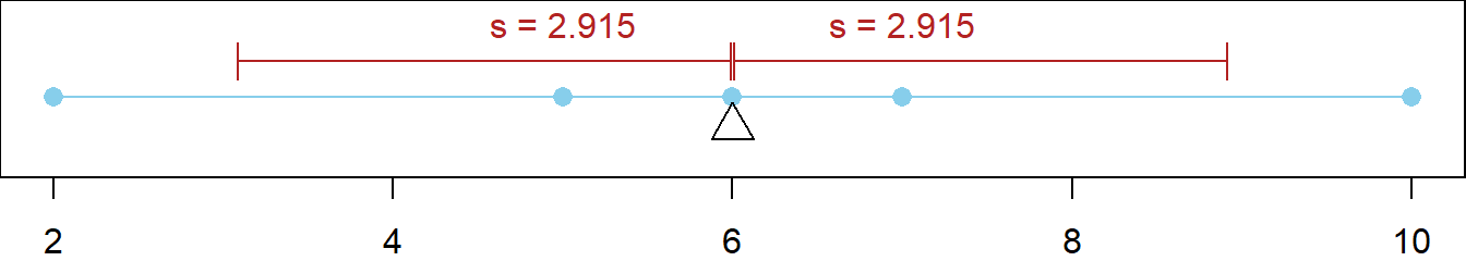
An Example

Say there are five data points given by

$x_1 = 2$
$x_2 = 5$
$x_3 = 6$
$x_4 = 7$
$x_5 = 10$

The mean of these values is $\bar{x}=6$ as shown here.

The five deviations are

$(x_1 - \bar{x}) = (2 - 6) = -4$
$(x_2 - \bar{x}) = (5 - 6) = -1$
$(x_3 - \bar{x}) = (6 - 6) = 0$
$(x_4 - \bar{x}) = (7 - 6) = 1$
$(x_5 - \bar{x}) = (10 - 6) = 4$

The squared deviations are

$(x_1 - \bar{x})^2 = (2 - 6)^2 = (-4)^2 = 16$
$(x_2 - \bar{x})^2 = (5 - 6)^2 = (-1)^2 = 1$
$(x_3 - \bar{x})^2 = (6 - 6)^2 = (0)^2 = 0$
$(x_4 - \bar{x})^2 = (7 - 6)^2 = (1)^2 = 1$
$(x_5 - \bar{x})^2 = (10 - 6)^2 = (4)^2 = 16$

The sum of the squared deviations is

\[ \sum_{i=1}^n (x_i-\bar{x})^2 = 16 + 1 + 0 + 1 + 16 = 34 \]

Dividing this by the degrees of freedom, $n-1$, gives

\[ \frac{\sum_{i=1}^n (x_i-\bar{x})^2}{n-1} = \frac{34}{5-1} = \frac{34}{4} = 8.5 \]

Finally, $s$ is obtained by taking the square root

\[ s = \sqrt{\frac{\sum_{i=1}^n(x_i-\bar{x})^2}{n-1}} = \sqrt{8.5} \approx 2.915 \]

The red lines below show how the standard deviation represents all deviations in this data set. Recall that the magnitudes of the individual deviations were $4, 1, 0, 1$, and $4$. The representative deviation is $2.915$.

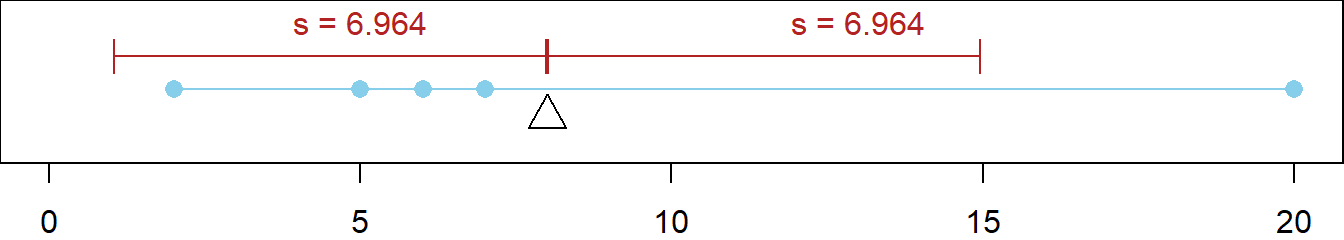
Effect of Outliers

Like the mean, the standard deviation is influenced by outliers. This is shown below by changing $x_5$ to be 20. Note that the deviation of $x_5$ is now 12 (instead of 4 like it was previously) and that the mean is now $8$ (as shown here). The standard deviation of the altered data

$x_1 = 2$
$x_2 = 5$
$x_3 = 6$
$x_4 = 7$
$x_5 = 20$

is now $s \approx 6.964$. Not very “representative” of all the deviations. It is biased towards the largest deviation. It is important to be aware of outliers when reporting the standard deviation $s$.

Variance

\[s^2 = \frac{\sum_{i=1}^n(x_i-\bar{x})^2}{n-1}\]

Measure of Spread | 1 Quantitative Variable

Overview

Great theoretical properties, but seldom used when describing data. Difficult to interpret in context of data because it is in squared units. The standard deviation is typically used instead because it is in the original units and is thus easier to interpret.

R Instructions

To calculate the variance in R use the code:

var(object)

object must be a quantitative variable, what R calls a “numeric vector.”

Example Code

Hover your mouse over the example codes to learn more.

var “var” is an R function used to calculate the variance of data. ( Parenthesis to begin the function. Must touch the last letter of the function. airquality “airquality” is a dataset. Type “View(airquality)” in R to see it. $ The $ allows us to access any variable from the airquality dataset. Temp “Temp” is a quantitative variable (numeric vector) from the “airquality” dataset. )
Closing parenthsis for the function.
Press Enter to run the code if you have typed it in yourself. You can also click here to view the output. … Click to View Output.

## [1] 89.59133

Note that the single number showing above is the variance of Temp from the airquality dataset.

library(tidyverse) tidyverse is an R Package that is very useful for working with data.
airquality airquality is a dataset in R. %>% The pipe operator that will send the airquality dataset down inside of the code on the following line.
group_by( “group_by” is a function from library(tidyverse) that allows us to split the airquality dataset into “little” datasets, one dataset for each value in the “Month” column. Month “Month” is a column from the airquality dataset that can be treated as qualitative. ) Functions must always end with a closing parenthesis. %>% The pipe operator that will send the grouped version of the airquality dataset down inside of the code on the following line.
summarise( “summarise” is a function from library(tidyverse) that allows us to compute numerical summaries on data. varTemp = “varTemp” is just a name we made up. It will contain the results of the var(…) function. var( “var” is an R function used to calculate the variance Temp Temp is a quantitative variable (numeric vector) from the airquality dataset. ) Functions must always end with a closing parenthesis. ) Functions must always end with a closing parenthesis.
Press Enter to run the code. … Click to View Output.

## `summarise()` ungrouping output (override with `.groups` argument)

Month	varTemp
5	46.99
6	43.54
7	18.62
8	43.37
9	69.82

Note that R calculated the variance of Temp for each month in Month from the airquality dataset.

May (5), June (6), July (7), August (8), and September (9), respectively.

Range

\[x_{(n)}-x_{(1)}\]

Measure of Spread | 1 Quantitative Variable

Overview

The difference between the maximum and minimum values. A general rule of thumb is that the range divided by four is roughly the standard deviation. Quick to obtain, but not as good as using the standard deviation. Was used more frequently before the advent of modern calculators.

R Instructions

R will not automatically compute the range. It is easiest to compute the max() and min() and perform the subtraction max - min yourself.

To calculate the variance in R use the code:

var(object)

object must be a quantitative variable, what R calls a “numeric vector.”

Example Code

Hover your mouse over the example codes to learn more.

max “max” is an R function used to calculate the maximum of data. ( Parenthesis to begin the function. Must touch the last letter of the function. airquality “airquality” is a dataset. Type “View(airquality)” in R to see it. $ The $ allows us to access any variable from the airquality dataset. Temp “Temp” is a quantitative variable (numeric vector) from the “airquality” dataset. )
Closing parenthsis for the function. - Subtraction symbol. min “min” is an R function used to calculate the minimum of data. ( Parenthesis to begin the function. Must touch the last letter of the function. airquality “airquality” is a dataset. Type “View(airquality)” in R to see it. $ The $ allows us to access any variable from the airquality dataset. Temp “Temp” is a quantitative variable (numeric vector) from the “airquality” dataset. )
Closing parenthsis for the function.
Press Enter to run the code if you have typed it in yourself. You can also click here to view the output. … Click to View Output.

## [1] 41

Note that the single number showing above is the range of Temp from the airquality dataset.

library(tidyverse) tidyverse is an R Package that is very useful for working with data.
airquality airquality is a dataset in R. %>% The pipe operator that will send the airquality dataset down inside of the code on the following line.
group_by( “group_by” is a function from library(tidyverse) that allows us to split the airquality dataset into “little” datasets, one dataset for each value in the “Month” column. Month “Month” is a column from the airquality dataset that can be treated as qualitative. ) Functions must always end with a closing parenthesis. %>% The pipe operator that will send the grouped version of the airquality dataset down inside of the code on the following line.
summarise( “summarise” is a function from library(tidyverse) that allows us to compute numerical summaries on data. rangeTemp = “rangeTemp” is just a name we made up. It will contain the results of the range calculation. max( “max” is an R function used to calculate the maximum Temp Temp is a quantitative variable (numeric vector) from the airquality dataset. ) Functions must always end with a closing parenthesis. - Minus sign to perform subtraction. min( “min” is an R function used to calculate the minimum Temp Temp is a quantitative variable (numeric vector) from the airquality dataset. ) Functions must always end with a closing parenthesis. ) Functions must always end with a closing parenthesis.
Press Enter to run the code. … Click to View Output.

## `summarise()` ungrouping output (override with `.groups` argument)

Month	rangeTemp
5	25
6	28
7	19
8	25
9	30

Note that R calculated the range of Temp for each month in Month from the airquality dataset.

May (5), June (6), July (7), August (8), and September (9), respectively.

Percentile (Quantile)

$\leftarrow$To the Left

Measure of Location | 1 Quantitative Variable

Overview

The percent of data that is equal to or less than a given data point. Useful for describing the relative position of a data point within a data set. If the percentile is close to 100, then the observation is one of the largest. If it is close to zero, then the observation is one of the smallest.

R Instructions

To compute the quantile in R for a given percentile:

quantile(object, percentile)

object must be a quantitative variable, or as R terms it, a “numeric vector”.
percentile must be a value between 0 and 1 or a “numeric vector” of such values.

quantile( “quantile” is an R function used to calculate the data value corresponding to a given percentile. airquality$Temp Temp is a quantitative variable (numeric vector) being accessed from the airquality dataset with the $ sign. , Comma separating the two commands of the quantile function. 0.8 The value of 0.8 specifies the 80th percentile. Any other value from 0 to 1 inclusive could be used. ) Functions must always end with a closing parenthesis.
Press Enter to run the code. … Click to View Output.

## 80% 
##  86

The 80th percentile for Temp is shown in the output above.

Proportion

\[\hat{p}=\frac{x}{n}\]

Measure of Center | 1 Qualitative Variable

Overview

The percent of observations in the data that satisfy some requirement. Obtained by dividing the number of successes $x$ by the number of total observations $n$. Often referred to as a percentage.

Correlation

$r = \frac{\textstyle\sum\left(\frac{x-\bar{x}}{s_x}\right)\left(\frac{y-\bar{y}}{s_y}\right)}{n-1}$

Measure of Association | 2 Quantitative Variables

Overview

Describes the strength and direction of the association between two quantitative variables. Restricted to values between -1 and 1. A value of zero denotes no association between the two variables. A value of 1 or -1 implies a perfect positive or perfect negative association, respectively.

R Instructions

To calculate the correlation in R use the code:

cor(object1,object2)

object1 and object2 must both be a quantitative variables, what R calls “numeric vectors.”

Example Code

Hover your mouse over the example codes to learn more.

cor “cor” is an R function used to calculate the standard deviation of data. ( Parenthesis to begin the function. Must touch the last letter of the function. airquality “airquality” is a dataset. Type “View(airquality)” in R to see it. $ The $ allows us to access any variable from the airquality dataset. Temp “Temp” is a quantitative variable (numeric vector) from the “airquality” dataset. , The comma is needed to separate the two quantitative variables of the cor() function. The space after the comma is not required. It just looks nice. airquality “airquality” is a dataset. Type “View(airquality)” in R to see it. $ The $ allows us to access any variable from the airquality dataset. Wind “Wind” is a quantitative variable (numeric vector) from the “airquality” dataset. )
Closing parenthsis for the function.
Press Enter to run the code if you have typed it in yourself. You can also click here to view the output. … Click to View Output.

## [1] -0.4579879

Note that the single number showing next to the [1] above is the correlation of Temp and Wind from the airquality dataset.

library(tidyverse) tidyverse is an R Package that is very useful for working with data.
airquality airquality is a dataset in R. %>% The pipe operator that will send the airquality dataset down inside of the code on the following line.
group_by( “group_by” is a function from library(tidyverse) that allows us to split the airquality dataset into “little” datasets, one dataset for each value in the “Month” column. Month “Month” is a column from the airquality dataset that can be treated as qualitative. ) Functions must always end with a closing parenthesis. %>% The pipe operator that will send the grouped version of the airquality dataset down inside of the code on the following line.
summarise( “summarise” is a function from library(tidyverse) that allows us to compute numerical summaries on data. corTempWind = “corTempWind” is just a name we made up. It will contain the results of the cor(…) function. cor( “cor” is an R function used to calculate the mean. Temp, Temp is a quantitative variable (numeric vector) from the airquality dataset. Wind Wind is a quantitative variable (numeric vector) from the airquality dataset. ) Functions must always end with a closing parenthesis. ) Functions must always end with a closing parenthesis.
Press Enter to run the code. … Click to View Output.

## `summarise()` ungrouping output (override with `.groups` argument)

Month	corTempWind
5	-0.3733
6	-0.121
7	-0.3052
8	-0.5076
9	-0.5705

Note that R calculated the correlation of Temp and Wind for each Month from the airquality dataset.